TotalDepth Command Line Tools
This describes the command line tools that are available for processing any TotalDepth file.
The tools are located in TotalDepth/
Plotting Well Logs
These command line tools plot wireline data.
PlotLogs.py
Produces SVG plots from LIS and LAS files.
Usage
Usage:
usage: PlotLogs.py [-h] [--version] [-j JOBS] [-k] [-l LOGLEVEL] [-g] [-r]
                   [-A] [-x LGFORMAT] [-X LGFORMAT_MIN] [-s SCALE]
                   in out
Arguments
These are required arguments unless -h or --version options are specified (in which case no processing is done):
- The path to the input LAS or LIS file or directory thereof.
- The path to the output SVG file or directory, any directories will be created as necessary.
Options
| Option | Description |
|---|---|
| --version | Show program’s version number and exit |
| -h, --help | Show this help message and exit. |
| -j JOBS, --jobs=JOBS | Max processes when multiprocessing. Zero uses number of native CPUs [8]. -1 disables multiprocessing. [default: -1] |
| -k, --keep-going | Keep going as far as sensible. [default: False] |
| -l LOGLEVEL, --loglevel=LOGLEVEL | Log Level (debug=10, info=20, warning=30, error=40, critical=50) [default: 20] |
| -g, --glob | File pattern match. [default none] |
| -r, --recursive | Process input recursively. [default: False] |
| -A, --API | Put an API header on each plot. [default: False] |
| -x LGFORMAT, --xml LGFORMAT | Use XML LgFormat UniqueId to use for plotting (additive). Use -x? to see what LgFormats (UniqueID+Description) are available. Use -x?? to see what curves each format can plot. See also -X. This is additive so can used multiple times to get multiple plots from the same data. |
| -X LGFORMAT_MIN, --XML LGFORMAT_MIN | Use all available LgFormat XML plots that use LGFORMAT_MIN or more outputs. If -x option present limited by those LgFormats [default: 0] |
| -s SCALE, --scale SCALE | Scale of X axis to use (an integer). This overrides the scale(s) specified in the LgFormat file or FILM table. [default: 0]. |
Examples
LgFormat XML
Using -x? to see what formats are available:
$ python3 PlotLogs.py -x? spam eggs
The output is something like:
Cmd: PlotLogs.py -x? spam eggs
XML LgFormats available: [29]
UniqueId                              Description
-----------------------------------   --------------------------------
ADN_Image_Format                    : ADN Image Log
Azimuthal_Density_3Track.xml        : Azimuthal Density 3Track
Azimuthal_Resistivity_3Track.xml    : Azimuthal Resistivity 3Track
Blank_3Track_Depth                  : Blank 3Track
Blank_3Track_Time.xml               : Blank 3Track Time
FMI_IMAGE_ALIGNED                   : FMI Image Aligned
FMI_IMAGE_PROCESSED                 : FMI Image Processed
Formation_Test                      : Formation Test Time
HDT                                 : High Definition Dipmeter
Micro_Resistivity_3Track.xml        : Micro Resistivity 3 Track Format
Natural_GR_Spectrometry_3Track.xml  : Natural GR Spectrometry 3Track
OBMI_IMAGE_EQUAL                    : OBMI Image Equalized
Porosity_GR_3Track                  : Standard Porosity Curves
Pulsed_Neutron_3Track.xml           : Pulsed Neutron 3Track
Pulsed_Neutron_Time.xml             : Pulsed Neutron Time
RAB_Image_Format_Deep               : Resistivity At the Bit Image
RAB_Image_Format_Medium             : Resistivity At the Bit Image
RAB_Image_Format_Shallow            : Resistivity At the Bit Image
RAB_Std_Format                      : Resistivity At the Bit
Resistivity_3Track_Correlation.xml  : Resistivity Linear Correlation Format
Resistivity_3Track_Logrithmic.xml   : Logrithmic Resistivity 3Track
Resistivity_Investigation_Image.xml : AIT Radial Investigation Image
Sonic_3Track.xml                    : Sonic DT Porosity 3 Track
Sonic_PWF4                          : SONIC Packed Waveform 4
Sonic_SPR1_VDL                      : SONIC Receiver Array Lower Dipole VDL
Sonic_SPR2_VDL                      : SONIC Receiver Array Upper Dipole VDL
Sonic_SPR3_VDL                      : SONIC Receiver Array Stonely VDL
Sonic_SPR4_VDL                      : SONIC Receiver Array P and S VDL
Triple_Combo                        : Resistivity Density Neutron GR 3Track Format
The first column is the UniqueID to be used in identifying plots for the -x option.
Using -x?? to see what formats and what curves would be plotted by each plot specification:
$ python3 PlotLogs.py -x?? a b
The output is something like:
Cmd: PlotLogs.py -x?? a b
XML LgFormats available: [29]
UniqueId                              Description
-----------------------------------   --------------------------------
ADN_Image_Format                    : ADN Image Log
    DRHB, GR  , GR_RAB, ROBB, ROP5, TNPH
Azimuthal_Density_3Track.xml        : Azimuthal Density 3Track
    BS  , DCAL, DRHB, DRHL, DRHO, DRHR, DRHU, DTAB, HDIA, PEB , PEF , PEL
    PER , PEU , RHOB, ROBB, ROBL, ROBR, ROBU, ROP5, RPM , SCN2, SOAB, SOAL
    SOAR, SOAU, SONB, SOXB, VDIA
Azimuthal_Resistivity_3Track.xml    : Azimuthal Resistivity 3Track
    AAI , BS  , C1  , C2  , CALI, GR  , GRDN_RAB, GRLT_RAB, GRRT_RAB, GRUP_RAB, PCAL, RDBD
    RDBL, RDBR, RDBU, RLA0, RLA1, RLA2, RLA3, RLA4, RLA5, RMBD, RMBL, RMBR
    RMBU, ROP5, RPM , RSBD, RSBL, RSBR, RSBU, SP  , TENS
Blank_3Track_Depth                  : Blank 3Track
Blank_3Track_Time.xml               : Blank 3Track Time
FMI_IMAGE_ALIGNED                   : FMI Image Aligned
    C1  , C2  , GR  , HAZIM, P1AZ, SP  , TENS
FMI_IMAGE_PROCESSED                 : FMI Image Processed
    C1  , C2  , GR  , HAZIM, P1AZ, SP  , TENS
Formation_Test                      : Formation Test Time
    B1TR, BFR1, BQP1, BQP1, BQP1, BQP1, BSG1, POHP
HDT                                 : High Definition Dipmeter
    C1  , C2  , DEVI, FC0 , FC1 , FC2 , FC3 , FC4 , GR  , HAZI, P1AZ, RB
Micro_Resistivity_3Track.xml        : Micro Resistivity 3 Track Format
    BMIN, BMNO, BS  , CALI, GR  , HCAL, HMIN, HMNO, MINV, MLL , MNOR, MSFL
    PROX, RXO , SP  , TENS
Natural_GR_Spectrometry_3Track.xml  : Natural GR Spectrometry 3Track
    CGR , PCAL, POTA, ROP5, SGR , SIGM, TENS, THOR, URAN
OBMI_IMAGE_EQUAL                    : OBMI Image Equalized
    C1  , C1_OBMT, C2  , C2_OBMT, GR  , HAZIM, OBRA3, OBRB3, OBRC3, OBRD3, P1AZ, P1NO_OBMT
    TENS
Porosity_GR_3Track                  : Standard Porosity Curves
    APDC, APLC, APSC, BS  , C1  , C2  , CALI, CALI_CDN, CMFF, CMRP, DPHB, DPHI
    DPHZ, DPOR_CDN, DRHO, ENPH, GR  , HCAL, NPHI, NPOR, PCAL, RHOB, RHOZ, ROP5
    SNP , SP  , SPHI, TENS, TNPB, TNPH, TNPH_CDN, TPHI
Pulsed_Neutron_3Track.xml           : Pulsed Neutron 3Track
    FBAC, GR  , INFD, SIGM, TAU , TCAF, TENS, TPHI, TSCF, TSCN
Pulsed_Neutron_Time.xml             : Pulsed Neutron Time
    FBAC_SL, GR_SL, INFD_SL, SIGM_SL, TAU_SL, TCAF_SL, TENS_SL, TPHI_SL, TSCF_SL, TSCN_SL
RAB_Image_Format_Deep               : Resistivity At the Bit Image
    GR_RAB, RES_BD, RES_BM, RES_BS, RES_RING, ROP5
RAB_Image_Format_Medium             : Resistivity At the Bit Image
    GR_RAB, RES_BD, RES_BM, RES_BS, RES_RING, ROP5
RAB_Image_Format_Shallow            : Resistivity At the Bit Image
    GR_RAB, RES_BD, RES_BM, RES_BS, RES_RING, ROP5
RAB_Std_Format                      : Resistivity At the Bit
    AAI , BDAV, BDM3, BMAV, BMM2, BSAV, BSM1, BTAB, CALI, DEVI, GR_RAB, HAZI
    OBIT, RBIT, RING, ROP5, RPM , RTAB
Resistivity_3Track_Correlation.xml  : Resistivity Linear Correlation Format
    AHT20, AHT60, AHT90, ATR , BS  , CALI, CATR, CILD, CLLD, GR  , HCAL, ILD
    ILM , LLD , LLS , MSFL, PCAL, PSR , RLA0, ROP5, RT  , RXO , SFL , SP
    TENS
Resistivity_3Track_Logrithmic.xml   : Logrithmic Resistivity 3Track
    A22H, A34H, AHF10, AHF20, AHF30, AHF60, AHF90, AHO10, AHO20, AHO30, AHO60, AHO90
    AHT10, AHT20, AHT30, AHT60, AHT90, ATR , BS  , CALI, GR  , HCAL, ILD , ILM
    LLD , LLM , MSFL, P16H_RT, P28H_RT, P34H_RT, PCAL, PSR , RLA0, RLA1, RLA2, RLA3
    RLA4, RLA5, ROP5, RXO , SFL , SP  , TENS
Resistivity_Investigation_Image.xml : AIT Radial Investigation Image
    AHT10, AHT20, AHT30, AHT60, AHT90, BS  , GR  , HCAL, SP
Sonic_3Track.xml                    : Sonic DT Porosity 3 Track
    BS  , CALI, DT  , DT0S, DT1R, DT2 , DT2R, DT4S, DTBC, DTCO, DTCU, DTL
    DTLF, DTLN, DTR2, DTR5, DTRA, DTRS, DTSH, DTSM, DTST, DTTA, GR  , HCAL
    PCAL, ROP5, SP  , SPHI, TENS
Sonic_PWF4                          : SONIC Packed Waveform 4
    CALI, DT1 , DT2 , DTCO, DTSM, DTST, GR  , HCAL, TENS
Sonic_SPR1_VDL                      : SONIC Receiver Array Lower Dipole VDL
    CALI, DT1 , DT1 , DT2 , DTCO, DTSM, DTST, GR  , HCAL, TENS
Sonic_SPR2_VDL                      : SONIC Receiver Array Upper Dipole VDL
    CALI, DT1 , DT2 , DT2 , DTCO, DTSM, DTST, GR  , HCAL, TENS
Sonic_SPR3_VDL                      : SONIC Receiver Array Stonely VDL
    CALI, DT1 , DT2 , DT3R, DTCO, DTSM, DTST, GR  , HCAL, TENS
Sonic_SPR4_VDL                      : SONIC Receiver Array P and S VDL
    CALI, DT1 , DT2 , DTCO, DTRP, DTRS, DTSM, DTST, GR  , HCAL, TENS
Triple_Combo                        : Resistivity Density Neutron GR 3Track Format
    AHT10, AHT20, AHT30, AHT60, AHT90, APDC, APLC, APSC, ATR , BS  , C1  , C2
    CALI, CMFF, CMRP, DPHB, DPHI, DPHZ, DPOR_CDN, DSOZ, ENPH, GR  , HCAL, HMIN
    HMNO, ILD , ILM , LLD , LLM , MSFL, NPHI, NPOR, PCAL, PEFZ, PSR , RLA0
    RLA1, RLA2, RLA3, RLA4, RLA5, ROP5, RSOZ, RXO , RXOZ, SFL , SNP , SP
    SPHI, TENS, TNPB, TNPH, TNPH_CDN, TPHI
Plotting Logs
Here is an example of plotting LIS and LAS files in directory in/ with the plots in directory out/. The following options have been invoked:
- API headers on the top of each plot: -A
- Multiprocessing on with 4 simultaneous jobs: -j4
- Recursive search of input directory: -r
- Uses any available plot specifications from LgFormat XML files which result in 4 curves or more being plotted: -X 4
The command line is:
$ python3 PlotLogs.py -A -j4 -r -X 4 in/ out/
First PlotLogs.py echos the command:
Cmd: PlotLogs.py -A -j4 -r -X 4 in/ out/
When complete PlotLogs.py writes out a summary, first the number of files read (output is wrapped here with ‘\’ for clarity):
plotLogInfo PlotLogInfo <__main__.PlotLogInfo object at 0x101e0da90> \
        Files=23 \
        Bytes=10648531 \
        LogPasses=23 \
        Plots=8 \
        Curve points=229991
Then as summary of each plot in detail (output is wrapped here with ‘\’ for clarity):
('in/1003578128.las', \
        0, \
        'Natural_GR_Spectrometry_3Track.xml', \
        IndexTableValue( \
                scale=100, \
                evFirst='800.5 (FEET)', \
                evLast='3019.5 (FEET)', \
                evInterval='2219.0 (FEET)', \
                curves='CGR_2, POTA, SGR_1, TENS_16, THOR, URAN', \
                numPoints=26213, \
                outPath='out//1003578128.las_0000_Natural_GR_Spectrometry_3Track.xml.svg' \
        )
)
('in/1003578128.las', \
        0, \
        'Porosity_GR_3Track', \
        IndexTableValue( \
                scale=100, \
                evFirst='800.5 (FEET)', \
                evLast='3019.5 (FEET)', \
                evInterval='2219.0 (FEET)', \
                curves='Cali, DRHO, DensityPorosity, GammaRay, NeutronPorosity, OLDESTNeutronPorosity, OLDNeutronPorosity, RHOB, SP, SonicPorosity, Tension', \
                numPoints=46170, \
                outPath='out//1003578128.las_0000_Porosity_GR_3Track.svg' \
        )
)

... 8<------------- Snip ------------->8

('in/1006346987.las', \
        0, 'Sonic_3Track.xml', \
        IndexTableValue(
                scale=100, \
                evFirst='4597.5 (FEET)', \
                evLast='5799.5 (FEET)', \
                evInterval='1202.0 (FEET)', \
                curves='Caliper, DT, DTL_DDBHC, GammaRay, SonicPorosity, TENSION', \
                numPoints=14430, \
                outPath='out//1006346987.las_0000_Sonic_3Track.xml.svg' \
        )
)
The fields in each tuple are:
Input file name.
LogPass number in the file. For example “Repeat Section” might be 0 and “Main Log” 1.
LgFormat used for the plot (several plots my be generated from one LogPass).
- An IndexTableValue object (used to generate the index.html file) that has the following fields:
- Plot scale as an integer.
- First reading and units as an Engineering Value.
- Last reading and units as an Engineering Value.
- Log interval and units as an Engineering Value.
- List of curve names plotted.
- Total number of data points plotted.
- The ouput file.
Finally the total number of curve feet plotted and the time it took:
Interval*curves: EngVal: 121020.000 (FEET)
  CPU time =    0.043 (S)
Exec. time =   25.119 (S)
Bye, bye!
In this case (under Unix) the “CPU Time” is the cumulative amount of CPU time used. As we are using multiprocessing it is the CPU time of the parent process which is very small since it just invokes child processes. The Exec. time is the wall clock time between starting and finishing PlotLogs.py.
In the output directory will be an index.html file that has a table with the fields that duplicate those on the command line output. It looks like this:
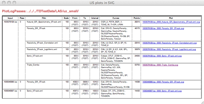
The links in the last column are to the SVG plots. Her is a screen shot of one:
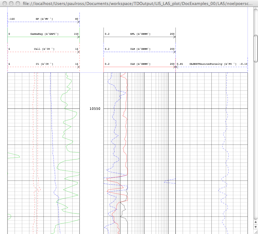
Sample Plots
Here is an actual plot from a LAS file and there are many more examples here: Wireline Plots.